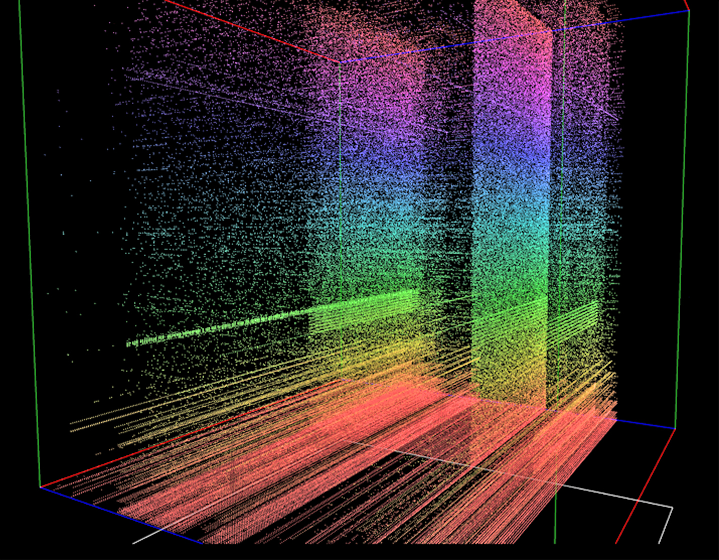
This is a screenshot taken with dotNetVis displaying 8,200,000 packets. A wide variety of malicious signatures can be seen in the image. There are creepy-crawly scans (The green horizontals), Port scans, lawnmower scans (the solid looking rectangles) and network sweeps (horizontal lines). This visualisation was generated using a Rhodes Network Telescope's capture file from 2009. About 6 months worth of data are represented in this image.
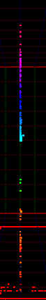
Barber pole scans occur across an array of hosts and they are harder to trace due to the fact that they vary their destination port number and destination host machine simultaneously. A text based intrusion detection system will have difficulty in identifying this kind of an attack, but when represented as a visualisation, such an attack is clearly visible. A barber pole signature is shown in alongside and it is identified by distinct diagonal lines.
Tools that are able to perform these scans are sophisticated in a sense that they have the ability to skip IP addresses and port numbers as well as scan more than one port on a target host. This flexibility decreases the detection rate as fuzzy patterns become more prominent.
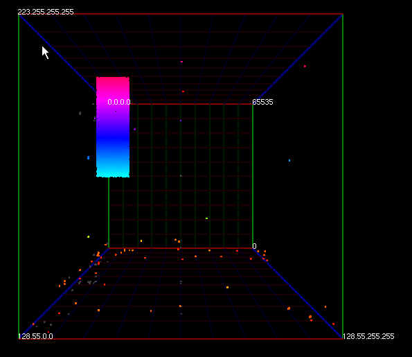
A port scan occurs on a single host. A port scan will usually report a list of open ports on the targeted machine. These ports are essentially tunnels into the secure host and with appropriate tools some ports can be used to gain unauthorised access into the host machine. A port scan can be identified by observing the traffic between a monitored node and the source IP address of the packets that that node is receiving. If a single source IP address is seen communicating to multiple ports on a host machine, then it is highly probable that a port scan is taking place.
There are many tools that can be used to carry out a port scan and some of the more clever tools attempt to be as discreet as possible. This makes it difficult to see the overall port scan signature as packets do not arrive uniformly. There are other methods that can be used to hide a port scan as well but that is beyond the scope of this thesis. A typical port scan is shown in alongside and it is a screenshot of a visualisation achieved using Lau's cube. A visible horizontal line is formed which indicates that a single source IP address has sent traffic to a multitude of port numbers on a single host.
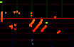
A lawnmower attack occurs across a wide range of contiguous ports and hosts. There is no discretion when one of these scans takes place. The tool used to initiate the scan will typically proceed to sequentially scan an address range by targeting a specific port identical to a port scan algorithm. Once the range has been traversed, the destination port is changed and the scan repeats. As shown alongside, the lawnmower scan signature is highly visible in a visualisation environment. The only difficulty in detecting a lawnmower scan is that the time it takes to execute is variable, as with any other scan. Because of this, the visualisation may decay before any visual signatures can be inferred.
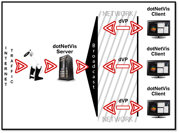
The figure alongside shows the enhanced structure implemented by the dotNetVis tool. The client-server model allows for multiple clients as well as independant and modularized components to allow for efficient processor and memory usage.
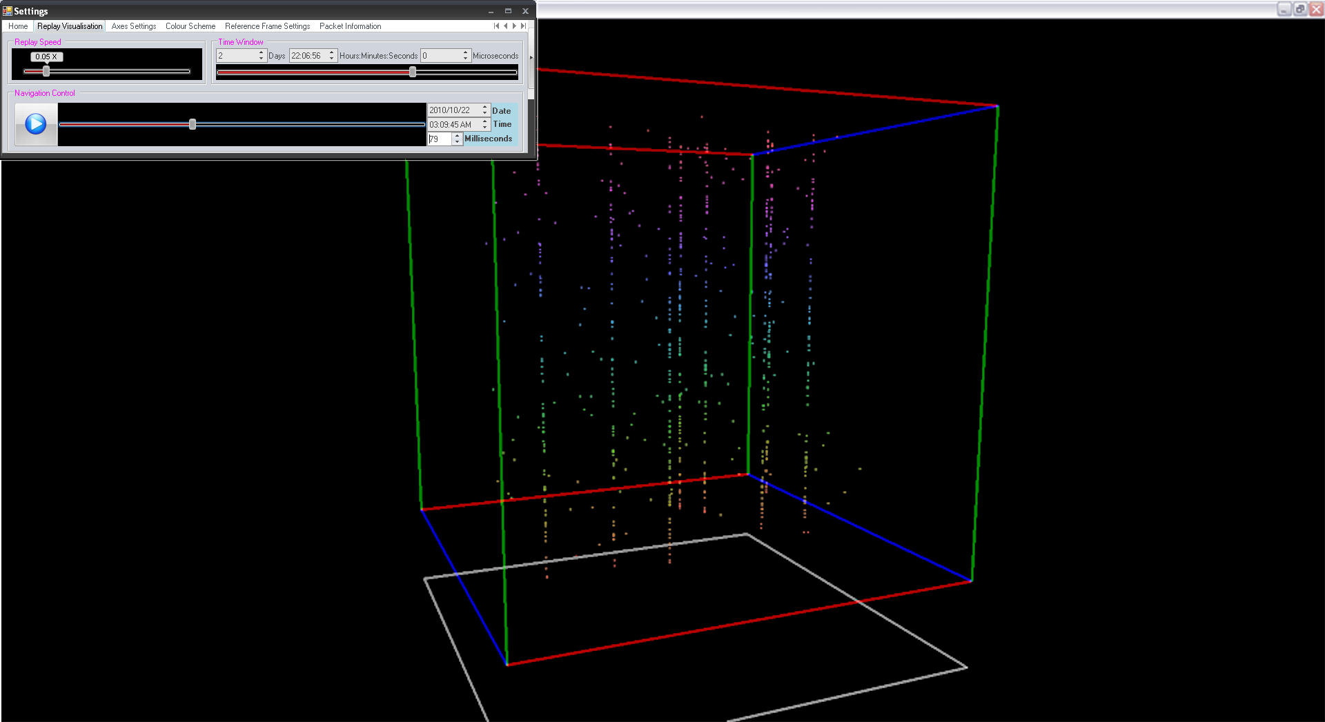
The visualisation alongside shows a dummy port scan that was rendered on a dotNetVis client computer. The diagonal lines are a distinct malicious signature which indicates a port scan from an external IP address. The image also shows the dotNetVis cube in fullscreen mode with the replay tab on the settings control active.
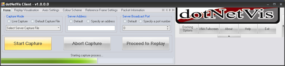
The home tab allows the user to configure the server connection settings, to select the network stream source for visualisation, and also to initiate the client server capture process. Once the process has been started, the underlying dVP library will be used to connect to the server using the specified settings and a capture request will be issued. When the capture process is started, a progress bar will relay the state of transmission.
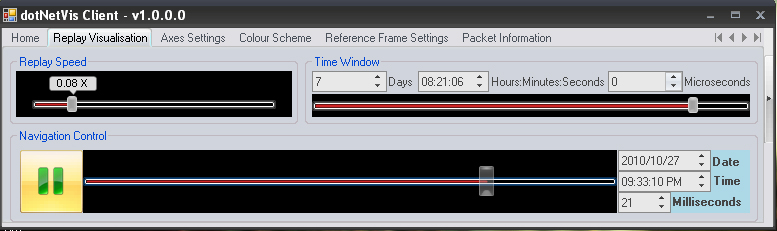
Replay of capture data will be controlled from this tab. The user can change the replay rate, set the time window indicating the range of data to be viewed simultaneously, and navigate through network events.
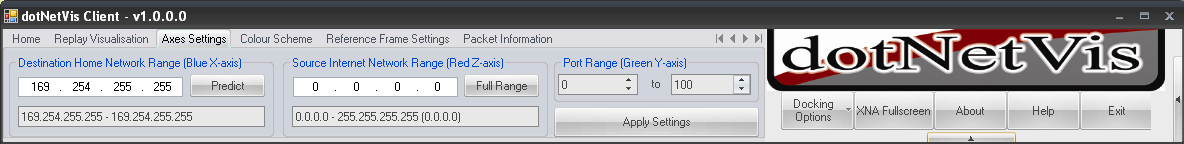
The configuration of axes settings is done through this tab. Set the destination range of the home network by either manually entering the range or by selecting the 'predict' button which will attempt to extrapolate the range from the capture file. The current implementation has no validity test to ensure that the correct range has been entered, so care should be taken when manually specifying the range. An incorrect range will simply yield an incorrect visualisation, either displaying no data or a subset of the full set. The destination address of a packet that is to be plotted will determine its position on the X-axis. Set the source internet network range in the same way as the destination range. This can be used to visualize a subset of the traffic in a capture file. The default value will monitor the entire address space. The source address of a packet that is to be plotted will determine its position relative to the Z-axis. This is used to specify a destination port range for monitoring. The destination port number of the IP network traffic that falls within the source and destination network ranges will be plotted on the Y-axis.
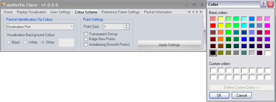
The default scheme is for the colours of plotted points to be chosen based on the destination port number value of the associated packet. Other options include using the protocol type, the destination or source address of packets to distinguish between the points. The background colour of the cube can be selected using the dropdown box or by selecting a common white or black setting. The visual representation can be enhanced by selecting an appropriate background colour based on the chosen colour settings and cube congestion. Point settings are included in the design but configuration has not been implemented due to a lack of support in XNA and time constraints.
The six sides of the cube, as well as the ICMP plane have the option of displaying a transparent grid that can be used to view the cube in segments rather than as a whole. A drop down checklist is used to toggle these grids. The opacity of the grids can be set to a value between 0 (being invisible) and 100. Each axis can be assigned a value which specifies the number of partitions the user wants the grid to be split into on that axis. This is done using the colour coded sliders. This helps to partition the cube nicely. The default value is 10 partitions on each axis. Text labels can be switched on for a more detailed representation. Axis labels show the ranges that have been selected and they also show the colours that have been assigned to the axes. A date and time label shows the current position of playback in the capture file. The framerate label gives an indication of the performance of the rendering component.
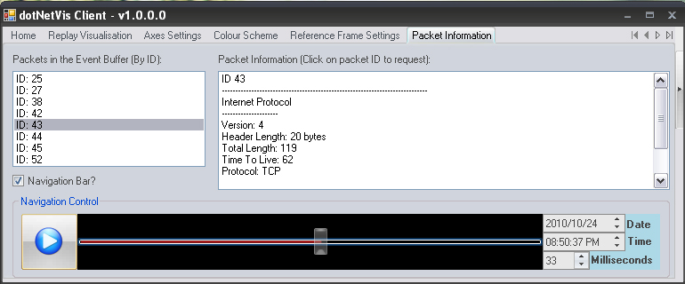
This tab is useful as it lists all the packets that are currently on display and that are in the event buffer. This list is updated on every frame. By scrolling over the items in the list of current packets, the user will be able to identify the relative packet in the cube. By selecting a packet in the list, that packet's information will be retrieved from the server and will be displayed in a second list. A pause and play toggle button is also available on this tab to allow for playback and navigation while concurrently observing the contents of the packet event buffer.